Introduction
This page compares the computational performance of
hesim against other R packages that have been
used to develop health economic models for health technology assessment.
We provide benchmarks for both a semi-Markov model and a
time-inhomogeneous Markov model.
The following R packages and scripts are used. The file
benchmarks.R contains the code used to run the models.
library("data.table")
library("flexsurv")
library("ggplot2")
library("heemod")
library("hesim")
library("kableExtra")
library("mstate")
source("benchmarks.R")
Semi-Markov models
Williams et
al. (2016) adapted the mstate
package to simulate parametric semi-Markov multi-state models. Here, we
use simulate a 6-state model for leukemia patients following bone marrow
transplantation with both hesim and mstate.
Since a semi-Markov process is assumed, an individual-level simulation
is used. Additional details were previously provided in a blog
post.
We fit a parametric Weibull model, but note that computational
performance does not differ substantially across parametric
distributions. We also checked the performance of a spline model, which
can be used to model very flexible baseline hazards, but is slower
because the quantile function must be computed numerically and
hesim, by default, uses inverse transform sampling to
randomly sample from survival splines. To facilitate direct comparison
with the Weibull model, we used a parameterization of the spline
equivalent to a Weibull distribution. When using mstate,
multi-state models are simulated using a cumulative hazard function
estimated on a discrete grid, so a time step must be defined. We used a
step size of 1/52 (i.e., one week) so that each time step was a week
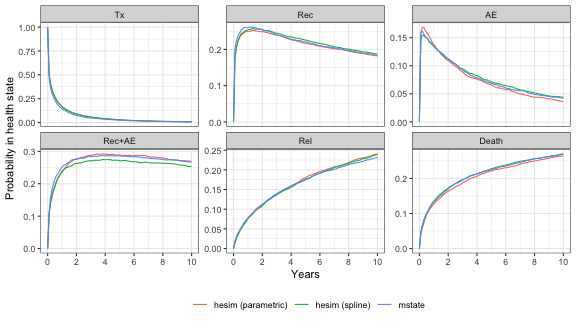
long. This produced reasonably accurate state probability estimates that
were similar to those performed in continuous time with
hesim (see plot below).
DIST = "weibull"
STEP = 1/52
We began by simulating “deterministic” models assuming no parameter
uncertainty. Comparisons of state probabilities simulated using 5,000
patients with hesim and mstate are shown in
the plot.
smb1 <-  benchmark_semi_markov(n_patients = 1000, uncertainty = "none", dist = DIST,
                               step = STEP)
smb2 <-  benchmark_semi_markov(n_patients = 5000, uncertainty = "none", dist = DIST,
                               step = STEP)
smb2$plot
We then performed probabilistic sensitivity analysis (PSA) and varied
both the number of patients simulated and the number of draws of the
parameters. Run times are reported in the table below.
hesim is considerably faster and the speed advantage is
most notable when a PSA is performed. Although slower than the Weibull
model, the spline model is still fast, meaning that flexible baseline
hazards can be modeled if required with only a small negative impact on
performance.
smb <- list(
  smb1,
  smb2,
  benchmark_semi_markov(n_patients = 1000, uncertainty = "normal",
                        n_samples = 100, dist = DIST,
                        step = STEP),
  benchmark_semi_markov(n_patients = 1000, uncertainty = "normal",
                        n_samples = 1000, dist = DIST,
                        step = STEP)
)
semi_markov_table(smb)| # of patients | # of PSA samples | mstate | hesim (parametric) | hesim (spline) |
|---|---|---|---|---|
| 1000 | 1 | 11 seconds | 0.062 seconds | 0.061 seconds |
| 5000 | 1 | 1.4 minutes | 0.11 seconds | 0.24 seconds |
| 1000 | 100 | 22 minutes | 0.63 seconds | 2.9 seconds |
| 1000 | 1000 | 3.6 hours | 6 seconds | 29 seconds |
Markov models
heemod
is a general purpose R package for simulating Markov cohort
models. We simulated the 5-state time inhomogeneous Markov model of
total hip replacement from the Decision
Modeling for Health Economic Evaluation textbook with
hesim and heemod. Vignettes for this example
are available in both packages ( hesim,
heemod).
Cohort models were simulated with both packages and an
individual-level model was also simulated with hesim. A
single representative patient was used in the cohort model and 1000
patients were simulated in the individual-level model. The cohort models
were simulated for 60 years using cycle lengths of 1 year.
mb <- list(
  benchmark_markov(n_samples = 10, n_patients = 1000),
  benchmark_markov(n_samples = 100, n_patients = 1000),
  benchmark_markov(n_samples = 1000, n_patients = 1000)
)
markov_table(mb)| # of PSA samples | Cohort | Individual | heemod | hesim (cohort) | hesim (individual) |
|---|---|---|---|---|---|
| 10 | 1 | 1000 | 1.5 seconds | 0.097 seconds | 0.21 seconds |
| 100 | 1 | 1000 | 12 seconds | 0.12 seconds | 1.1 seconds |
| 1000 | 1 | 1000 | 2 minutes | 1.2 seconds | 11 seconds |
Computing environment
## R version 4.0.3 (2020-10-10)
## Platform: x86_64-apple-darwin17.0 (64-bit)
## Running under: macOS Mojave 10.14.6
##
## Matrix products: default
## BLAS:   /Library/Frameworks/R.framework/Versions/4.0/Resources/lib/libRblas.dylib
## LAPACK: /Library/Frameworks/R.framework/Versions/4.0/Resources/lib/libRlapack.dylib
##
## locale:
## [1] en_US.UTF-8/en_US.UTF-8/en_US.UTF-8/C/en_US.UTF-8/en_US.UTF-8
##
## attached base packages:
## [1] stats     graphics  grDevices utils     datasets  methods   base
##
## other attached packages:
## [1] mstate_0.3.1      kableExtra_1.2.1  hesim_0.5.0.9999  heemod_0.13.0
## [5] ggplot2_3.3.3     flexsurv_1.1.1    survival_3.2-7    data.table_1.13.6
## [9] knitr_1.30
##
## loaded via a namespace (and not attached):
##  [1] deSolve_1.28       tidyselect_1.1.0   xfun_0.18          purrr_0.3.4
##  [5] splines_4.0.3      lattice_0.20-41    colorspace_2.0-0   vctrs_0.3.6
##  [9] generics_0.1.0     htmltools_0.5.0    viridisLite_0.3.0  rlang_0.4.10
## [13] pillar_1.4.7       glue_1.4.2         withr_2.3.0        RColorBrewer_1.1-2
## [17] pryr_0.1.4         muhaz_1.2.6.1      lifecycle_0.2.0    plyr_1.8.6
## [21] stringr_1.4.0      munsell_0.5.0      gtable_0.3.0       rvest_0.3.6
## [25] mvtnorm_1.1-1      mvnfast_0.2.5      codetools_0.2-16   evaluate_0.14
## [29] memoise_1.1.0      highr_0.8          Rcpp_1.0.5         scales_1.1.1
## [33] webshot_0.5.2      digest_0.6.27      stringi_1.5.3      dplyr_1.0.2
## [37] grid_4.0.3         quadprog_1.5-8     tools_4.0.3        magrittr_2.0.1
## [41] lazyeval_0.2.2     tibble_3.0.4       crayon_1.3.4       tidyr_1.1.2
## [45] pkgconfig_2.0.3    ellipsis_0.3.1     Matrix_1.2-18      xml2_1.3.2
## [49] rmarkdown_2.4      httr_1.4.2         rstudioapi_0.13    R6_2.5.0
## [53] compiler_4.0.3