Overview
The time inhomogeneous Markov individual-level modeling vignette shows how to simulate a continuous times state transition model (CTSTM) and perform a cost-effectiveness analysis (CEA). The model was parameterized using a variety of disparate data sources and parameter estimates. However, in an ideal scenario, a CTSTM can be fully parameterized by estimating a single statistical model. In this example, we demonstrate by fitting a multi-state model—a generalization of a survival model with more than two states—using patient-level data.
An example 3-state model
The reversible illness-death model is a commonly used state transition model (see figure below) with 3 health states and 4 transitions. In this example, we will use 3 generic health states: (1) Healthy, (2) Sick, and (3) Death. The following 4 transitions are possible.
- Healthy to Sick
- Sick to Healthy
- Healthy to Death
- Sick to Death

In general, the transitions of a multi-state model can be characterized with an H x H transition matrix where is the number of health states, which is a square-matrix where the (r,s) element is a positive integer if a transition from r to s is possible and NA otherwise. A 4 x 4 transition matrix is appropriate for the reversible illness death model.
tmat <- rbind(c(NA, 1, 2),
              c(3, NA, 4),
              c(NA, NA, NA))
colnames(tmat) <- rownames(tmat) <- c("Healthy", "Sick", "Death")
print(tmat)
## Healthy Sick Death
## Healthy NA 1 2
## Sick 3 NA 4
## Death NA NA NAIn a cost-effectiveness analysis, the treatments strategies of interest and characteristics of the target population must be specified in addition to the selected model structure. We will consider a simple case with two treatment strategies (the standard of care (SOC) and a new intervention) and a heterogeneous population of 1000 patients who differ by age and sex. The model contains 3 health states (2 of which are non-death states).
library("hesim")
library("data.table")
strategies <- data.table(strategy_id = c(1, 2),
                         strategy_name = c("SOC", "New"))
n_patients <- 1000
patients <- data.table(patient_id = 1:n_patients,
                       age = rnorm(n_patients, mean = 45, sd = 7),
                       female = rbinom(n_patients, size = 1, prob = .51))
states <- data.table(state_id = c(1, 2),
                     state_name = rownames(tmat)[1:2]) # Non-death health states
hesim_dat <- hesim_data(strategies = strategies,
                        patients = patients,
                        states = states)
We will create nice labels for the plots and summary tables.
labs <- get_labels(hesim_dat)
labs$transition_id <- c("Healthy-> Sick" = 1,
                        "Healthy -> Death" = 2,
                        "Sick -> Healthy" = 3,
                        "Sick -> Death" = 4)
print(labs)
## $strategy_id
## SOC New
## 1 2
##
## $state_id
## Healthy Sick Death
## 1 2 3
##
## $transition_id
## Healthy-> Sick Healthy -> Death Sick -> Healthy Sick -> Death
## 1 2 3 4Parameter estimation
Multi-state model
CTSTMs can be parameterized by fitting statistical models in
R or by storing the parameters from a model fit outside
R as described in the introduction to
hesim. Either a single joint model can be estimated
encompassing all transitions or separate models can be estimated for
each possible transition. In the introduction we considered a
joint model; here, we will fit separate models. A number of parametric
and flexibly parametric approaches are available (as described more
detail in the params_surv() documentation), but we will
illustrate with a Weibull model.
We will begin by fitting a “clock reset” model using
flexsurvreg().
library("flexsurv")
n_trans <- max(tmat, na.rm = TRUE) # Number of transitions
wei_fits_cr <- vector(length = n_trans, mode = "list")
for (i in 1:length(wei_fits_cr)){
  wei_fits_cr[[i]] <- flexsurvreg(Surv(years, status) ~ factor(strategy_id),
                                  data = mstate3_exdata$transitions,
                                  subset = (trans == i) ,
                                  dist = "weibull")
}
wei_fits_cr <- flexsurvreg_list(wei_fits_cr)
“Clock forward” models are fit in a similar fashion by specifying
both the starting (Tstop) and stopping (Tstop)
times associated with each transition.
wei_fits_cf <- vector(length = n_trans, mode = "list")
for (i in 1:length(wei_fits_cf)){
  wei_fits_cf[[i]] <- flexsurvreg(Surv(Tstart, Tstop, status) ~ factor(strategy_id),
                                  data = mstate3_exdata$transitions,
                                  subset = (trans == i) ,
                                  dist = "weibull")
}
wei_fits_cf <- flexsurvreg_list(wei_fits_cf)
Utility and costs
The most straightforward way to assign utility and cost values to
health states is with a stateval_tbl(). For example, we can
specify the mean and standard error of utilities by health state
(implying that utility values do not vary by treatment strategy or
patient) and that we will use a beta distribution to randomly sample
utility values for the probabilistic sensitivity analysis (PSA).
utility_tbl <- stateval_tbl(data.table(state_id = states$state_id,
                                       mean = mstate3_exdata$utility$mean,
                                       se = mstate3_exdata$utility$se),
                            dist = "beta")
head(utility_tbl)
## state_id mean se
## <num> <num> <num>
## 1: 1 0.65 0.1732051
## 2: 2 0.85 0.2000000Drug and medical costs can be specified in a similar fashion. Drug costs are assumed to be known with certainty and vary by treatment strategy whereas medical costs are assumed to vary by health state and to follow a gamma distribution.
drugcost_tbl <- stateval_tbl(data.table(strategy_id = strategies$strategy_id,
                                       est = mstate3_exdata$costs$drugs$costs),
                            dist = "fixed")
medcost_tbl <- stateval_tbl(data.table(state_id = states$state_id,
                                       mean = mstate3_exdata$costs$medical$mean,
                                       se = mstate3_exdata$costs$medical$se),
                            dist = "gamma")
Simulation
Constructing the economic model
As in any hesim model, the economic model consists of a
model for disease progression and models for assigning utility and cost
values to health states. In this example, we will use 1000 samples of
the parameters for the probabilistic sensitivity analysis (PSA).
n_samples <- 1000Disease model
We begin by constructing the model for health state transitions,
which is a function of input data (i.e., covariates) and a fitted
multi-state model (or a parameter object). When separate multi-state
models are fit by transition, the input data consists of one observation
for each treatment strategy and patient combination (joint models
consist of one observation for each treatment strategy, patient, and
transition combination). It can be created easily by using the
expand() function to expand the hesim_data()
object created above.
##    strategy_id patient_id strategy_name      age female
##          <num>      <int>        <char>    <num>  <int>
## 1:           1          1           SOC 35.19970      1
## 2:           1          2           SOC 46.78722      0
## 3:           1          3           SOC 27.93915      1
## 4:           1          4           SOC 44.96100      1
## 5:           1          5           SOC 49.35087      0
## 6:           1          6           SOC 53.03888      1
“Clock reset” and “clock forward” transition models are created by combining the fitted models and input data with the transition matrix, desired number of PSA samples, the timescale of the model, and the starting age of each patient in the simulation (by default, patients are assumed to live no longer than age 100 in the individual-level simulation).
transmod_cr <- create_IndivCtstmTrans(wei_fits_cr, transmod_data,
                                      trans_mat = tmat, n = n_samples,
                                      clock = "reset",
                                      start_age = patients$age)
transmod_cf <- create_IndivCtstmTrans(wei_fits_cf, transmod_data,
                                      trans_mat = tmat, n = n_samples,
                                      clock = "forward",
                                      start_age = patients$age)
It is a good idea to evaluate the assumptions underlying multi-state
models. hesim can help facilitate these analyses since
hazards ($hazard()), cumulative hazards
($cumhazard()), and state probabilities
($stateprobs()) can be easily computed. As an illustration,
we will predict hazards using the maximum likelihood estimates of the
Weibull model for a single patient (patient_id = 1). To do
so, we create new transition models based on a subset of the dataset
transmod_data used above.
# Predict hazard
transmod_data_pat1 <- transmod_data[patient_id == 1]
predict_haz <- function(fits, clock){
 transmod_cr_pat1 <- create_IndivCtstmTrans(fits, transmod_data_pat1,
                                            trans_mat = tmat,
                                            clock = clock,
                                            uncertainty = "none")
  haz <- transmod_cr_pat1$hazard(t = seq(0, 20, 1))
  title_clock <- paste(toupper(substr(clock, 1, 1)),
                       substr(clock, 2, nchar(clock)), sep="")
  haz[, clock := title_clock]
  return(haz[, ])
}
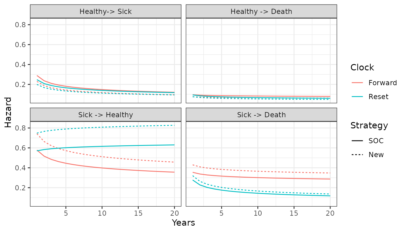
We then plot the predicted hazard by treatment strategy and timescale.
# Plot hazards
library("ggplot2")
haz <- rbind(predict_haz(wei_fits_cr, "reset"),
             predict_haz(wei_fits_cf, "forward"))
set_labels(haz, labels = labs,
           new_names = c("strategy_name", "trans_name"))
ggplot(haz[t > 0],
       aes(x = t, y = hazard, col = clock, linetype = strategy_name)) +
  geom_line() +
  facet_wrap(~trans_name) +
  xlab("Years") + ylab("Hazard") +
  scale_linetype_discrete(name = "Strategy") +
scale_color_discrete(name = "Clock") 
While the hazards from the healthy state are similar between the “clock forward” and “clock reset” approaches, they differ significantly in the sick state. Treatment effects (i.e., the hazard ratios between treatment strategies 1 and 2) are also largest in the sick state.
Additional analyses should be conducted as well. For instance, the
hazards for treatment strategy 1 (the reference treatment strategy)
could be assessed by comparing the Weibull model’s predictions with
predictions from non-parametric (i.e., the Kaplan-Meier estimator) or
semi-parametric (i.e., Cox) models. This can be performed using
mstate, which can predict cumulative hazards and state
probabilities in non-parametric and semi-parametric models. Furthermore,
the Weibull model’s proportional hazards assumption should be tested
using standard techniques such as plots of log time vs. the log
cumulative hazard, inclusion of time-dependent covariates, and tests of
the Schoenfeld residuals.
Utility and cost models
Cost and utility models can be easily created from the
stateval_tbl() output above. Note that these models are
based on predicted means (see tparams_mean()) and do depend
on covariates.
# Utility
utilitymod <- create_StateVals(utility_tbl, n = n_samples, hesim_data = hesim_dat)

# Costs
drugcostmod <- create_StateVals(drugcost_tbl, n = n_samples, hesim_data = hesim_dat)
medcostmod <- create_StateVals(medcost_tbl, n = n_samples, hesim_data = hesim_dat)
costmods <- list(Drug = drugcostmod,
                 Medical = medcostmod)
Combining the disease progression, cost, and utility models
Now that the necessary transition, utility, and cost models have been created, we combine them to create separate economic models based on the “clock reset” and “clock forward” transition models, respectively.
econmod_cr <- IndivCtstm$new(trans_model = transmod_cr,
                             utility_model = utilitymod,
                             cost_models = costmods)
econmod_cf <- IndivCtstm$new(trans_model = transmod_cf,
                             utility_model = utilitymod,
                             cost_models = costmods)
Simulating outcomes
Disease progression
Disease progression can be simulated using the
$sim_disease() method. In the individual-level simulation,
unique trajectories through the multi-state model are simulated for each
patient, treatment strategy, and PSA sample. Patients transition
from an old health state that was entered at time
time_start to a new health state at time
time_stop.
# "Clock reset"
econmod_cr$sim_disease()
head(econmod_cr$disprog_)
## sample strategy_id patient_id grp_id from to final time_start time_stop
## <num> <int> <int> <int> <num> <num> <int> <num> <num>
## 1: 1 1 1 1 1 3 1 0.000000 8.739756
## 2: 1 1 2 1 1 2 0 0.000000 2.492639
## 3: 1 1 2 1 2 1 0 2.492639 5.323266
## 4: 1 1 2 1 1 2 0 5.323266 5.607200
## 5: 1 1 2 1 2 1 0 5.607200 5.665132
## 6: 1 1 2 1 1 2 0 5.665132 5.665978
# "Clock forward"
econmod_cf$sim_disease()
State occupancy probabilities at different time points are computed
using $sim_stateprobs(). First, we simulate state
probabilities for the “clock reset” model.
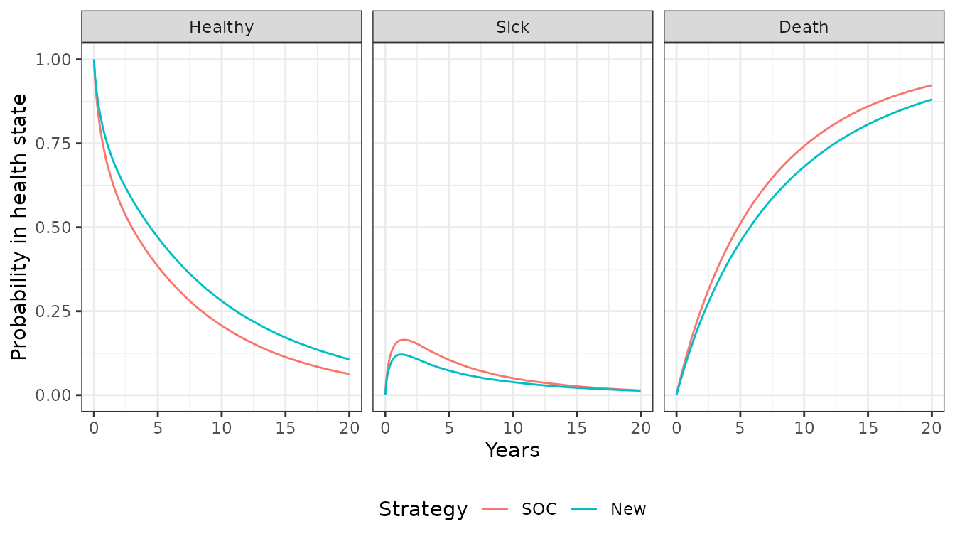
econmod_cr$sim_stateprobs(t = seq(0, 20 , 1/12)) We can then compare state probabilities between the competing treatment strategies.
# Short function to create state probability "dataset" for plotting
summarize_stprobs <- function(stateprobs){
  x <- stateprobs[, .(prob_mean = mean(prob)),
                  by = c("strategy_id", "state_id", "t")]
  set_labels(x, labels = labs, new_names = c("strategy_name", "state_name"))
}

# Plot of state probabilities
stprobs_cr <- summarize_stprobs(econmod_cr$stateprobs_)
ggplot(stprobs_cr, aes(x = t, y = prob_mean, col = strategy_name)) +
  geom_line() + facet_wrap(~state_name) +
  xlab("Years") + ylab("Probability in health state") +
  scale_color_discrete(name = "Strategy") +
theme(legend.position = "bottom") 
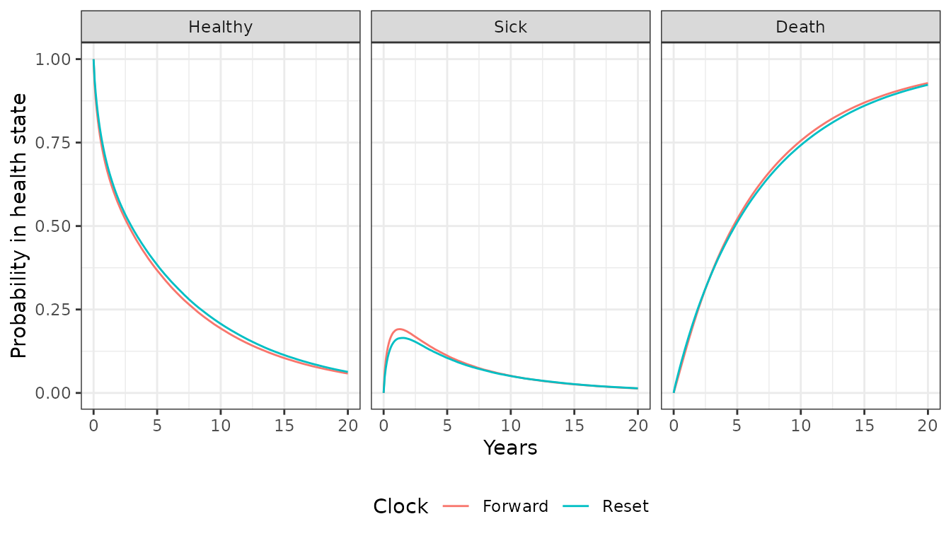
Next, we compare the state probabilities from the “clock reset” and “clock forward” models.
econmod_cf$sim_stateprobs(t = seq(0, 20 , 1/12))
stprobs_cf <- summarize_stprobs(econmod_cf$stateprobs_)

# Compare "clock forward" and "clock reset" cases
stprobs <- rbind(data.table(stprobs_cf, clock = "Forward"),
                 data.table(stprobs_cr, clock = "Reset"))
ggplot(stprobs[strategy_id == 1],
       aes(x = t, y = prob_mean, col = clock)) +
  geom_line() + facet_wrap(~state_name) +
  xlab("Years") + ylab("Probability in health state") +
  scale_color_discrete(name = "Clock") +
theme(legend.position = "bottom") 
The probabilities are generally quite similar, implying that the choice of timescale has a small impact on the results. This is not unexpected given that patients spend considerably more time in the healthy state and the predicted hazard rates are very similar in the healthy state.
Costs and QALYs
QALYs (and life-years) are simulated using $sim_qalys().
By default, mean QALYs are computed by treatment strategy, health state,
and PSA sample (the by_patient option can be used to
compute QALYs at the patient level). Here, we used the “clock reset”
model to compute both undiscounted QALYs (dr = 0) and QALYs
discounted at 3%.
##    sample strategy_id grp_id state_id    dr    qalys      lys
##     <num>       <int>  <int>    <num> <num>    <num>    <num>
## 1:      1           1      1        1     0 5.177696 6.241736
## 2:      1           1      1        2     0 1.310995 1.359593
## 3:      1           2      1        1     0 5.624203 6.780001
## 4:      1           2      1        2     0 1.132789 1.174782
## 5:      2           1      1        1     0 3.960689 5.963536
## 6:      2           1      1        2     0 1.663871 1.663871
Let’s compute means (across the PSA samples) by treatment strategy and health state to see how much each health state contributes to total QALYs.
qalys_summary <- econmod_cr$qalys_[, .(mean = mean(qalys)),
                                    by = c("strategy_id", "state_id", "dr")]
set_labels(qalys_summary, labels = labs,
           new_names = c("strategy_name", "state_name"))
ggplot(qalys_summary[dr == .03],
       aes(x = strategy_name, y = mean, fill = state_name)) +
  geom_bar(stat = "identity") +
  scale_fill_discrete(name = "") +
xlab("Strategy") + ylab("Mean QALYs") 
Costs are computed in the same way as QALYs, except that they are computed by category. We use the “clock reset” model and a 3% discount rate.
econmod_cr$sim_costs(dr = 0.03)
head(econmod_cr$costs_)
## sample strategy_id grp_id state_id dr category costs
## <num> <int> <int> <num> <num> <char> <num>
## 1: 1 1 1 1 0.03 Drug 25259.931
## 2: 1 1 1 2 0.03 Drug 5483.400
## 3: 1 2 1 1 0.03 Drug 54341.846
## 4: 1 2 1 2 0.03 Drug 9422.090
## 5: 2 1 1 1 0.03 Drug 24348.012
## 6: 2 1 1 2 0.03 Drug 6789.699Decision analysis
Once costs and QALYs are computed a cost-effectiveness analysis can
be performed. The $summarize() method creates a
hesim::ce object with mean costs and QALYs computed for
each PSA sample and summary results are produced with
summary.ce(). The cea() and
cea_pw() can then be used for cost-effectiveness analysis
as described in the cost-effectiveness analysis
vignette.
##    Discount rate        Outcome                     SOC                     New
##            <num>         <fctr>                  <char>                  <char>
## 1:          0.00          QALYs       5.12 (2.74, 7.19)       6.10 (3.17, 9.07)
## 2:          0.03          QALYs       4.13 (2.23, 5.70)       4.72 (2.51, 6.81)
## 3:          0.03    Costs: Drug 30,008 (25,533, 34,838) 69,865 (57,940, 82,467)
## 4:          0.03 Costs: Medical    6,697 (5,690, 7,718)    7,514 (6,265, 8,818)
## 5:          0.03   Costs: total 36,705 (31,205, 42,589) 77,379 (64,289, 91,308)