Markov models with multinomial logistic regression

Overview

When discrete time data is collected at evenly spaced intervals, cohort discrete time state transition models (cDTSTMs)—often referred to as Markov cohort models—can be parameterized using multinomial logistic regression. Separate multinomial logit model are estimated for each health state and predict the probability of transitioning from that state to all other states. Mathematically, the probability of a transition from state $r$ at model cycle $t$ to state $s$ at model cycle $t+1$ is given by,

$Pr(y_{t+1} = s| y_t = r) = \frac{e^{x_r\beta_{rs}}}{\sum_{h=1}^{H}e^{x_r\beta_{rh}}}$

An example 3-state model

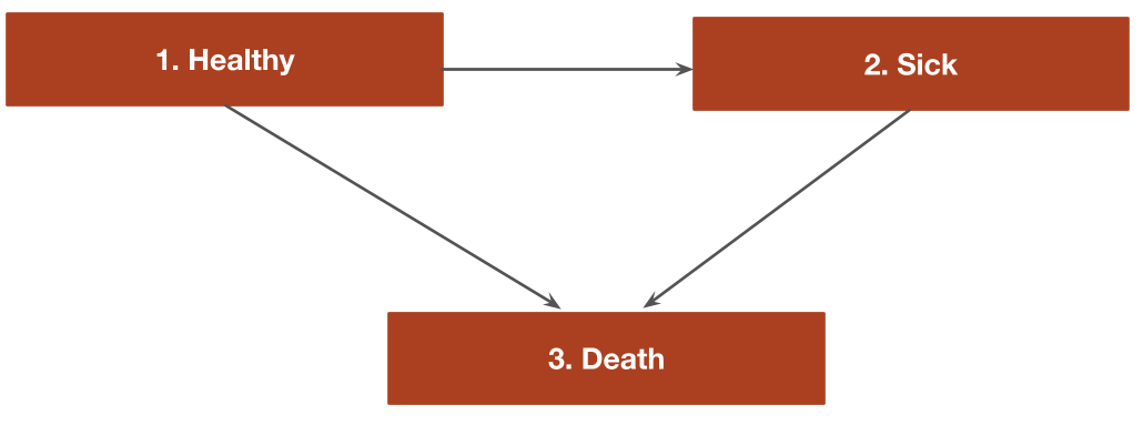
We illustrate by considering an illness-death model with 3 generic health states: (1) Healthy, (2) Sick, and (3) Death We will assume that patients can only transition to a more severe health state:

Healthy to Sick
Healthy to Death
Sick to Death

The transitions of this model can be characterized with a transition matrix with the number of rows and columns equal to the number of health states. In the multinomial logistic regression case, the reference category in each multinomial logit fit is assigned a value of zero. Elements representing transitions that are not possible are NA. All other transitions are represented with integer values from 1 to $K_r -1$ where $K_r$ is the number of states in the multinomial logit model for state $r$ .

tmat <- rbind(c(0, 1, 2),
              c(NA, 0, 1),
              c(NA, NA, NA))
colnames(tmat) <- rownames(tmat) <- c("Healthy", "Sick", "Death")
print(tmat)

##         Healthy Sick Death
## Healthy       0    1     2
## Sick         NA    0     1
## Death        NA   NA    NA

The cost-effectiveness analysis will compare two treatment strategies—the “Intervention” and the “Reference” treatment. Separate multinomial logistic regressions are fit for patients starting in the healthy state and the sick state using the multinom3_exdata example dataset, which tracks patient health states at yearly time intervals in a longitudinal fashion.

library("hesim")
library("data.table")
transitions_data <- data.table(multinom3_exdata$transitions)
head(transitions_data)

##    patient_id strategy_id strategy_name      age        age_cat female  year
##         <int>       <int>        <fctr>    <num>         <fctr>  <int> <num>
## 1:          1           1     Reference 37.68882       Age < 40      0     1
## 2:          2           1     Reference 20.17811       Age < 40      0     1
## 3:          3           1     Reference 62.81725      Age >= 60      0     1
## 4:          4           2  Intervention 58.12408 40 <= Age < 60      0     1
## 5:          5           2  Intervention 30.72299       Age < 40      1     1
## 6:          6           1     Reference 33.49259       Age < 40      0     1
##    state_from state_to year_cat
##        <fctr>   <fctr>   <fctr>
## 1:    Healthy     Sick Year < 3
## 2:    Healthy  Healthy Year < 3
## 3:    Healthy  Healthy Year < 3
## 4:    Healthy     Dead Year < 3
## 5:    Healthy     Sick Year < 3
## 6:    Healthy  Healthy Year < 3

In a typical Markov cohort model, either a single cohort or a small number of cohorts is simulated. However, one advantage of using an explicit statistical model to predict transition probabilities is that a large heterogeneous cohort of patients can be easily simulated. Here, we will simulate 100 representative patients (i.e., cohorts), which arguably better captures the underlying heterogeneity in the population. To do so, we will randomly sample 100 patients from the multinom3_exdata dataset. In our data, we observe differences in age and gender.

n_patients <- 100
patients <- transitions_data[year == 1, .(patient_id, age, female)][
  sample.int(nrow(transitions_data[year == 1]), n_patients)][
  , grp_id := 1:n_patients]
head(patients)

##    patient_id      age female grp_id
##         <int>    <num>  <int>  <int>
## 1:       5293 19.71306      0      1
## 2:       5527 88.87563      1      2
## 3:       6604 90.16717      1      3
## 4:        485 18.88980      0      4
## 5:       2607 85.22011      1      5
## 6:       1476 19.70745      0      6

To perform the cost-effectiveness analysis, each patient is simulated twice, once with the reference treatment and once with the intervention. The non-death states use for simulating costs and quality-adjusted life-years (QALYs) are the healthy and sick states.

hesim_dat <- hesim_data(
  patients = patients,
  strategies = data.table(strategy_id = 1:2,
                          strategy_name = c("Reference", "Intervention")),
  states = data.table(state_id = c(1, 2),
                     state_name = rownames(tmat)[1:2]) # Non-death health states
)

We can use get_labels() to create nice labels for the plots and summary tables.

labs <- get_labels(hesim_dat)
print(labs)

## $strategy_id
##    Reference Intervention 
##            1            2 
## 
## $state_id
## Healthy    Sick   Death 
##       1       2       3

Parameter estimation

Multinomial logit model for transition probabilities

hesim can simulate cDTSTMs with transition probabilities fit via multinomial logistic regression with the nnet package. The probability of a health state transition is modeled as a function of the treatment strategy, patient age, and gender. The nonlinear impact of age is modeled using a natural spline with splines::ns(). In addition, time period indicator variables (year_cat) are included so that transition probabilities can change over time, which makes the Markov model time inhomogeneous.

library("nnet")
library("splines")

# Transitions from healthy state
data_healthy <- transitions_data[state_from == "Healthy"]
fit_healthy <- multinom(state_to ~ strategy_name + female + 
                          ns(age, df = 5) + year_cat, 
                        data = data_healthy, trace = FALSE)

# Transitions from sick state
data_sick <- droplevels(transitions_data[state_from == "Sick"])
fit_sick <- multinom(state_to ~ strategy_name + female + 
                       ns(age, df = 5) + year_cat, 
                     data = data_sick, trace = FALSE)

The separate fits are stored in a list to facilitate prediction of the transition probability matrix.

transfits <- multinom_list(healthy = fit_healthy, sick = fit_sick)

Utility and costs

As in the simple Markov cohort and time inhomogeneous Markov cohort modeling vignettes, utility and costs models could be generated using mathematical expressions with define_model(). However, in this case it is simpler and more direct (and thus more computationally efficient) to use the stateval_tbl() functionality. Separate tables are created for utility, drug costs, and medical costs.

utility_tbl <- stateval_tbl(multinom3_exdata$utility,
                            dist = "beta")
head(utility_tbl)

##    state_id state_name  mean        se
##       <num>     <char> <num>     <num>
## 1:        1    Healthy  0.90 0.1732051
## 2:        2       Sick  0.65 0.2000000

drugcost_tbl <- stateval_tbl(multinom3_exdata$costs$drugs,
                            dist = "fixed")
medcost_tbl <- stateval_tbl(multinom3_exdata$costs$medical,
                            dist = "gamma")

Simulation

The economic model consists of a model for disease progression and models for assigning utility and cost values to health states. Since we are performing a PSA, we must specify the number of times to sample the parameters.

n_samples <- 100

Constructing the economic model

Disease model

The disease model can be easily constructed from our fitted multinomial logistic regression models and input data. The input data has one observation for each treatment strategy and patient. In addition, since we included time period dummies, we separate the covariates into distinct time intervals in order to make the model time inhomogeneous.

tintervals <- time_intervals(unique(transitions_data[, .(year_cat)])
                             [, time_start := c(0, 2, 6)])
transmod_data <- expand(hesim_dat, times = tintervals)
transmod <- create_CohortDtstmTrans(transfits,
                                    input_data = transmod_data,
                                    trans_mat = tmat,
                                    n = n_samples,
                                    uncertainty = "normal")

Utility and cost models

The utility and cost models can be created directly from the utility and cost tables since they do not include covariates. That is, unlike the disease model which explicitly models the transition probabilities as a function of covariates, they are based solely on predicted means (see tparams_mean()) and therefore do not require input data.

# Utility
utilitymod <- create_StateVals(utility_tbl, n = n_samples, hesim_data = hesim_dat)

# Costs
drugcostmod <- create_StateVals(drugcost_tbl, n = n_samples, hesim_data = hesim_dat)
medcostmod <- create_StateVals(medcost_tbl, n = n_samples, hesim_data = hesim_dat)
costmods <- list(Drug = drugcostmod,
                 Medical = medcostmod)

Combining the disease progression, cost, and utility models

The transition, utility, and cost models are combined to create the cDTSTM.

econmod <- CohortDtstm$new(trans_model = transmod,
                           utility_model = utilitymod,
                           cost_models = costmods)

Simulating outcomes

Disease progression

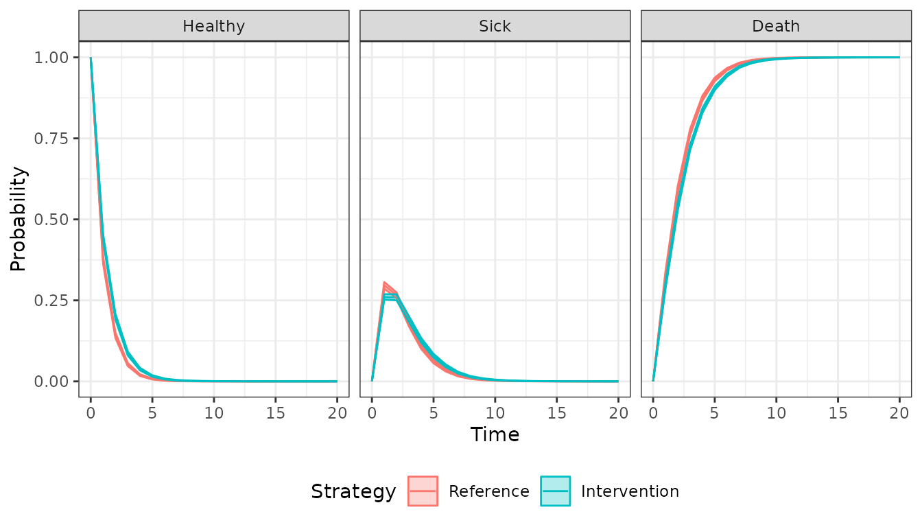
We simulate state probabilities over 20 years with 1-year model cycles. autoplot.stateprobs() is used to plot the probability of being in each of the 3 states over the model’s time horizon, with the solid lines representing means from the PSA and the shaded regions representing 95% confidence intervals.

econmod$sim_stateprobs(n_cycles = 20)
autoplot(econmod$stateprobs_, labels = labs,
         ci = TRUE, ci_style = "ribbon")

Costs and QALYs

After simulating the health state transitions, costs and QALYs are simulated in a straightforward manner. As is typical, we use a 3 percent discount rate.

econmod$sim_qalys(dr = .03)
econmod$sim_costs(dr = .03)

Decision analysis

Now that costs and QALYs have been simulated with the PSA, a decision analysis can be performed. We will focus on the pairwise comparison between the “Intervention” and the “Reference” treatment.

ce_sim <- econmod$summarize(by_grp = TRUE)
cea_pw_out <- cea_pw(ce_sim, comparator = 1, dr_qalys = .03, dr_costs = .03)

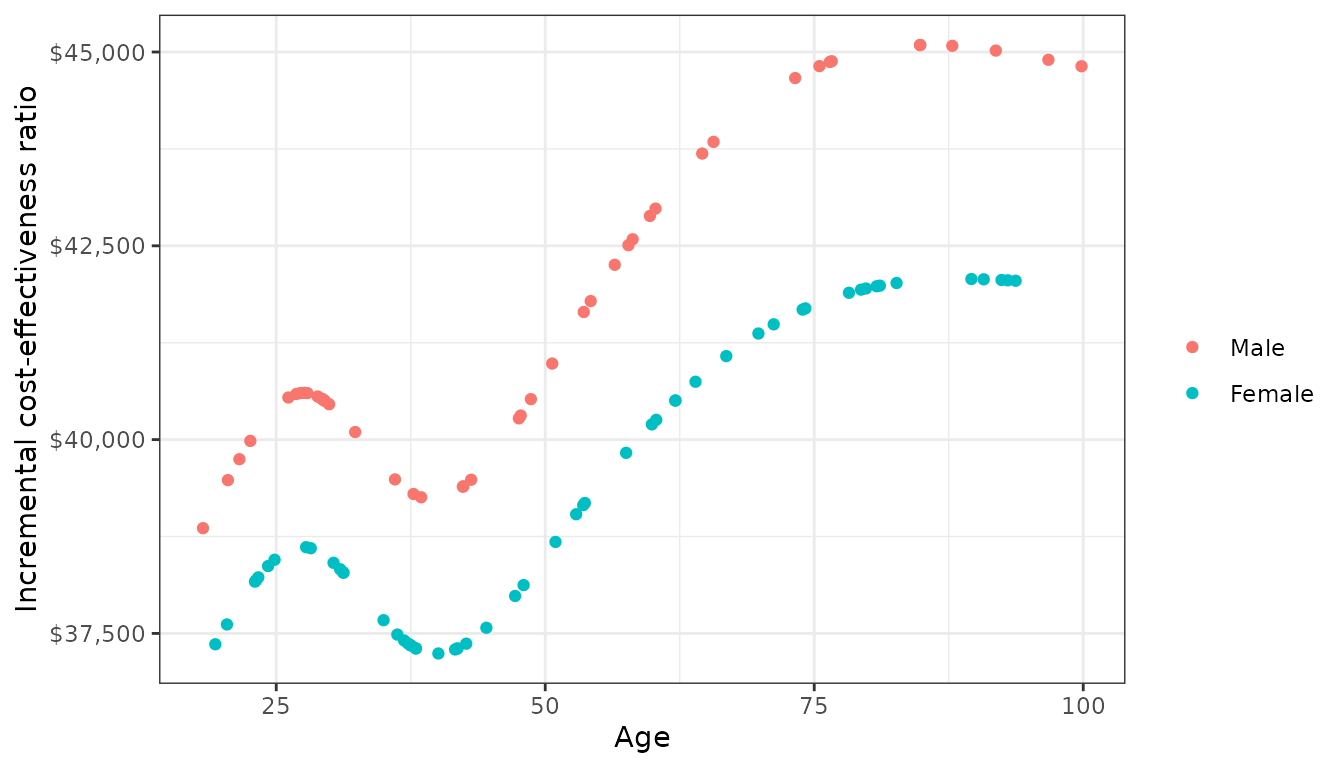
Since we modeled the health state transitions as a function of covariates, transition rates vary by patient characteristics. The impact of gender and the (nonlinear) impact of age on transitions have a similar effect on the incremental cost-effectiveness ratio (ICER). The ICERs were lower for females and tended to rise with age, suggesting that the “Intervention” was more effective for patients with a lower baseline risk.

icers <- merge(cea_pw_out$summary,
               hesim_dat$patients[, .(grp_id, age, female)],
               by = "grp_id")
icers[, gender := factor(female, 
                         levels = c(0, 1),
                         labels = c("Male", "Female"))]

# Plot of ICER by demographics
library("ggplot2")
ggplot(icers, aes(x = age, y = as.numeric(gsub(",", "", icer)), col = gender)) +
  geom_point() +
  xlab("Age") + ylab("Incremental cost-effectiveness ratio") +
  scale_y_continuous(label = scales::dollar_format()) +
  scale_colour_discrete(name = "") + 
  theme_bw()

Of note, the heterogeneous ICER arises completely through differences in baseline risk since the effect of the “Intervention” relative to the “Reference” on transitions was assumed to be constant across patients (i.e., the treatment strategy covariate did not have any effect modifiers). This example highlights an advantage of modeling disease progression with a statistical model in that it can facilitate analyses that assess the consequences of patient heterogeneity.

2024-09-18