Simulate outcomes from a cohort discrete time state transition model.
Format
An R6::R6Class object.
References
Incerti and Jansen (2021). See Section 2.1 for a description of a cohort DTSTM and details on simulating costs and QALYs from state probabilities. An example in oncology is provided in Section 4.3.
See also
CohortDtstm objects can be created from model objects as
documented in create_CohortDtstm(). The CohortDtstmTrans documentation
describes the class for the transition model and the StateVals documentation
describes the class for the cost and utility models. A CohortDtstmTrans
object is typically created using create_CohortDtstmTrans().
There are currently three relevant vignettes. vignette("markov-cohort")
details a relatively simple Markov model and
vignette("markov-inhomogeneous-cohort") describes a more complex time
inhomogeneous model in which transition probabilities vary in every model
cycle. The vignette("mlogit") shows how a transition model can be parameterized
using a multinomial logistic regression model when transition data is collected
at evenly spaced intervals.
Public fields
trans_modelThe model for health state transitions. Must be an object of class
CohortDtstmTrans.utility_modelThe model for health state utility. Must be an object of class
StateVals.cost_modelsThe models used to predict costs by health state. Must be a list of objects of class
StateVals, where each element of the list represents a different cost category.stateprobs_An object of class
stateprobssimulated using$sim_stateprobs().qalys_An object of class
qalyssimulated using$sim_qalys().costs_An object of class
costssimulated using$sim_costs().
Methods
Method new()
Create a new CohortDtstm object.
Usage
CohortDtstm$new(trans_model = NULL, utility_model = NULL, cost_models = NULL)Method sim_stateprobs()
Simulate health state probabilities using CohortDtstmTrans$sim_stateprobs().
Returns
An instance of self with simulated output of class stateprobs
stored in stateprobs_.
Method sim_qalys()
Simulate quality-adjusted life-years (QALYs) as a function of stateprobs_ and
utility_model. See sim_qalys() for details.
Usage
CohortDtstm$sim_qalys(
  dr = 0.03,
  integrate_method = c("trapz", "riemann_left", "riemann_right"),
  lys = TRUE
)
Arguments
drDiscount rate.
integrate_methodMethod used to integrate state values when computing costs or QALYs. Options are
trapzfor the trapezoid rule,riemann_leftfor a left Riemann sum, andriemann_rightfor a right Riemann sum.lysIf
TRUE, then life-years are simulated in addition to QALYs.
Returns
An instance of self with simulated output of class qalys stored
in qalys_.
Method sim_costs()
Simulate costs as a function of stateprobs_ and cost_models.
See sim_costs() for details.
Usage
CohortDtstm$sim_costs(
  dr = 0.03,
  integrate_method = c("trapz", "riemann_left", "riemann_right")
)
Arguments
drDiscount rate.
integrate_methodMethod used to integrate state values when computing costs or QALYs. Options are
trapzfor the trapezoid rule,riemann_leftfor a left Riemann sum, andriemann_rightfor a right Riemann sum.
Returns
An instance of self with simulated output of class costs stored
in costs_.
Method summarize()
Summarize costs and QALYs so that cost-effectiveness analysis can be performed.
See summarize_ce().
Examples
library("data.table")
library("ggplot2")
theme_set(theme_bw())
set.seed(102)
# NOTE: This example replicates the "Simple Markov cohort model"
# vignette using a different approach. Here, we explicitly construct
# the transition probabilities "by hand". In the vignette, the transition
# probabilities are defined using expressions (i.e., by using
# `define_model()`). The `define_model()` approach does (more or less) what
# is done here under the hood.
# (0) Model setup
hesim_dat <- hesim_data(
strategies = data.table(
strategy_id = 1:2,
strategy_name = c("Monotherapy", "Combination therapy")
),
patients <- data.table(patient_id = 1),
states = data.table(
state_id = 1:3,
state_name = c("State A", "State B", "State C")
)
)
n_states <- nrow(hesim_dat$states) + 1
labs <- get_labels(hesim_dat)
# (1) Parameters
n_samples <- 10 # Number of samples for PSA
## Transition matrix
### Input data (one transition matrix for each parameter sample,
### treatment strategy, patient, and time interval)
p_id <- tpmatrix_id(expand(hesim_dat, times = c(0, 2)), n_samples)
N <- nrow(p_id)
### Transition matrices (one for each row in p_id)
p <- array(NA, dim = c(n_states, n_states, nrow(p_id)))
#### Baseline risk
trans_mono <- rbind(
c(1251, 350, 116, 17),
c(0, 731, 512, 15),
c(0, 0, 1312, 437),
c(0, 0, 0, 469)
)
mono_ind <- which(p_id$strategy_id == 1 | p_id$time_id == 2)
p[,, mono_ind] <- rdirichlet_mat(n = 2, trans_mono)
#### Apply relative risks
combo_ind <- setdiff(1:nrow(p_id), mono_ind)
lrr_se <- (log(.710) - log(.365))/(2 * qnorm(.975))
rr <- rlnorm(n_samples, meanlog = log(.509), sdlog = lrr_se)
rr_indices <- list( # Indices of transition matrix to apply RR to
c(1, 2), c(1, 3), c(1, 4),
c(2, 3), c(2, 4),
c(3, 4)
)
rr_mat <- matrix(rr, nrow = n_samples, ncol = length(rr_indices))
p[,, combo_ind] <- apply_rr(p[, , mono_ind],
rr = rr_mat,
index = rr_indices)
tp <- tparams_transprobs(p, p_id)
## Utility
utility_tbl <- stateval_tbl(
data.table(
state_id = 1:3,
est = c(1, 1, 1)
),
dist = "fixed"
)
## Costs
drugcost_tbl <- stateval_tbl(
data.table(
strategy_id = c(1, 1, 2, 2),
time_start = c(0, 2, 0, 2),
est = c(2278, 2278, 2278 + 2086.50, 2278)
),
dist = "fixed"
)
dmedcost_tbl <- stateval_tbl(
data.table(
state_id = 1:3,
mean = c(A = 1701, B = 1774, C = 6948),
se = c(A = 1701, B = 1774, C = 6948)
),
dist = "gamma"
)
cmedcost_tbl <- stateval_tbl(
data.table(
state_id = 1:3,
mean = c(A = 1055, B = 1278, C = 2059),
se = c(A = 1055, B = 1278, C = 2059)
),
dist = "gamma"
)
# (2) Simulation
## Constructing the economic model
### Transition probabilities
transmod <- CohortDtstmTrans$new(params = tp)
### Utility
utilitymod <- create_StateVals(utility_tbl,
hesim_data = hesim_dat,
n = n_samples)
### Costs
drugcostmod <- create_StateVals(drugcost_tbl,
hesim_data = hesim_dat,
n = n_samples)
dmedcostmod <- create_StateVals(dmedcost_tbl,
hesim_data = hesim_dat,
n = n_samples)
cmedcostmod <- create_StateVals(cmedcost_tbl,
hesim_data = hesim_dat,
n = n_samples)
costmods <- list(drug = drugcostmod,
direct_medical = dmedcostmod,
community_medical = cmedcostmod)
### Economic model
econmod <- CohortDtstm$new(trans_model = transmod,
utility_model = utilitymod,
cost_models = costmods)
## Simulating outcomes
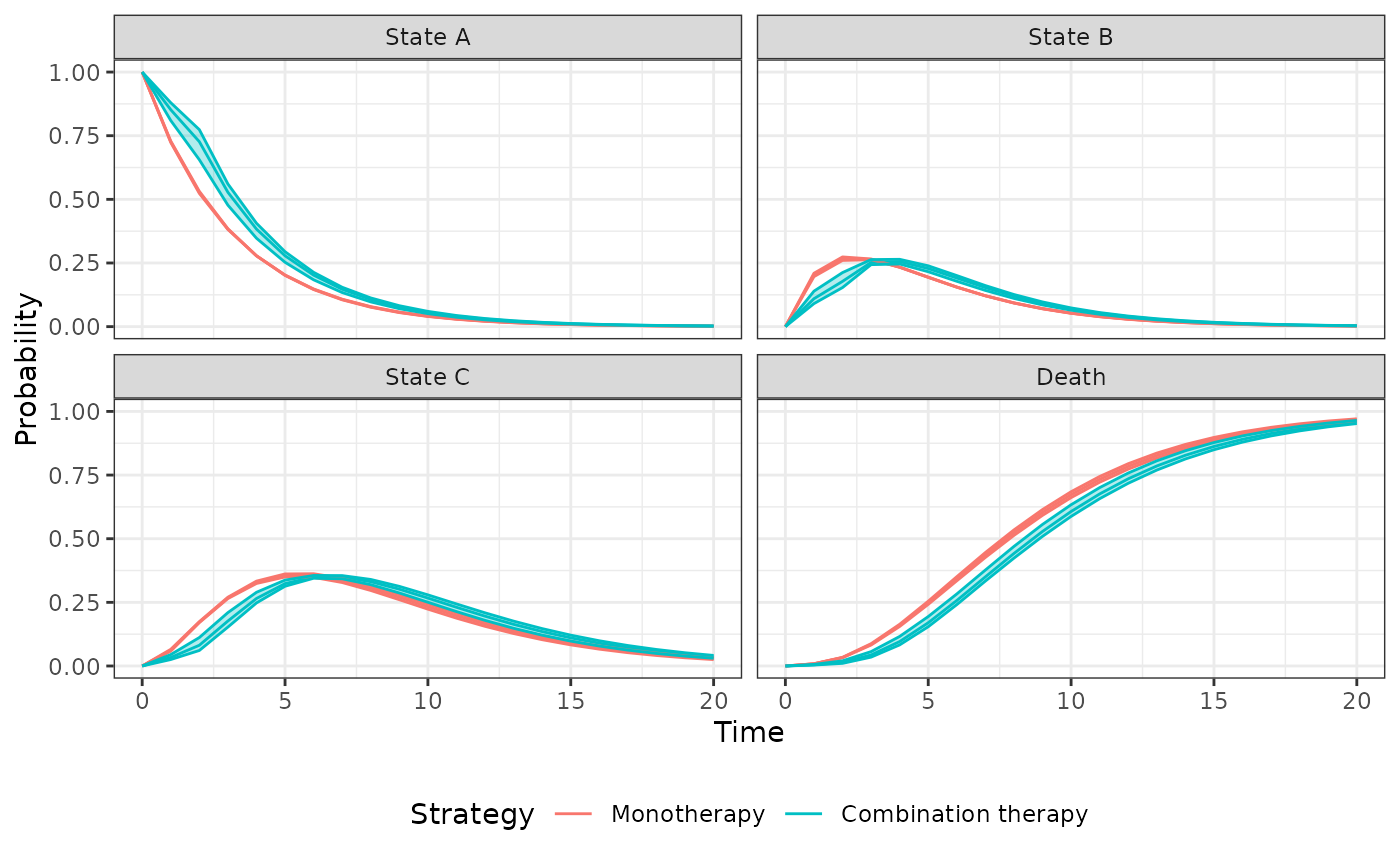
econmod$sim_stateprobs(n_cycles = 20)
autoplot(econmod$stateprobs_, ci = TRUE, ci_style = "ribbon",
labels = labs)
 econmod$sim_qalys(dr = 0, integrate_method = "riemann_right")
econmod$sim_costs(dr = 0.06, integrate_method = "riemann_right")
# (3) Decision analysis
ce_sim <- econmod$summarize()
wtp <- seq(0, 25000, 500)
cea_pw_out <- cea_pw(ce_sim, comparator = 1, dr_qalys = 0, dr_costs = .06,
k = wtp)
format(icer(cea_pw_out))
#> Outcome 2
#> <fctr> <char>
#> 1: Incremental QALYs 0.88 (0.42, 1.26)
#> 2: Incremental costs 5,252 (401, 8,617)
#> 3: Incremental NMB 38,957 (17,712, 56,120)
#> 4: ICER 5,940
econmod$sim_qalys(dr = 0, integrate_method = "riemann_right")
econmod$sim_costs(dr = 0.06, integrate_method = "riemann_right")
# (3) Decision analysis
ce_sim <- econmod$summarize()
wtp <- seq(0, 25000, 500)
cea_pw_out <- cea_pw(ce_sim, comparator = 1, dr_qalys = 0, dr_costs = .06,
k = wtp)
format(icer(cea_pw_out))
#> Outcome 2
#> <fctr> <char>
#> 1: Incremental QALYs 0.88 (0.42, 1.26)
#> 2: Incremental costs 5,252 (401, 8,617)
#> 3: Incremental NMB 38,957 (17,712, 56,120)
#> 4: ICER 5,940