Simulate outcomes from an N-state partitioned survival model.
Format
An R6::R6Class object.
References
Incerti and Jansen (2021). See Section 2.3 for a mathematical description of a PSM and Section 4.2 for an example in oncology. The mathematical approach used to simulate costs and QALYs from state probabilities is described in Section 2.1.
See also
The PsmCurves documentation
describes the class for the survival models and the StateVals documentation
describes the class for the cost and utility models. A PsmCurves
object is typically created using create_PsmCurves().
The PsmCurves documentation provides an example in which the model
is parameterized from parameter objects (i.e., without having the patient-level
data required to fit a model with R). A longer example is provided in
vignette("psm").
Public fields
survival_modelsThe survival models used to predict survival curves. Must be an object of class
PsmCurves.utility_modelThe model for health state utility. Must be an object of class
StateVals.cost_modelsThe models used to predict costs by health state. Must be a list of objects of class
StateVals, where each element of the list represents a different cost category.n_statesNumber of states in the partitioned survival model.
t_A numeric vector of times at which survival curves were predicted. Determined by the argument
tin$sim_curves().survival_An object of class survival simulated using
sim_survival().stateprobs_An object of class stateprobs simulated using
$sim_stateprobs().qalys_An object of class qalys simulated using
$sim_qalys().costs_An object of class costs simulated using
$sim_costs().
Methods
Method new()
Create a new Psm object.
Usage
Psm$new(survival_models = NULL, utility_model = NULL, cost_models = NULL)Method sim_stateprobs()
Simulate health state probabilities from survival_ using a partitioned
survival analysis.
Returns
An instance of self with simulated output of class stateprobs
stored in stateprobs_.
Method sim_qalys()
Simulate quality-adjusted life-years (QALYs) as a function of stateprobs_ and
utility_model. See sim_qalys() for details.
Usage
Psm$sim_qalys(
  dr = 0.03,
  integrate_method = c("trapz", "riemann_left", "riemann_right"),
  lys = TRUE
)
Arguments
drDiscount rate.
integrate_methodMethod used to integrate state values when computing costs or QALYs. Options are
trapzfor the trapezoid rule,riemann_leftfor a left Riemann sum, andriemann_rightfor a right Riemann sum.lysIf
TRUE, then life-years are simulated in addition to QALYs.
Returns
An instance of self with simulated output of class qalys stored
in qalys_.
Method sim_costs()
Simulate costs as a function of stateprobs_ and cost_models.
See sim_costs() for details.
Usage
Psm$sim_costs(
  dr = 0.03,
  integrate_method = c("trapz", "riemann_left", "riemann_right")
)
Arguments
drDiscount rate.
integrate_methodMethod used to integrate state values when computing costs or QALYs. Options are
trapzfor the trapezoid rule,riemann_leftfor a left Riemann sum, andriemann_rightfor a right Riemann sum.
Returns
An instance of self with simulated output of class costs stored
in costs_.
Method summarize()
Summarize costs and QALYs so that cost-effectiveness analysis can be performed.
See summarize_ce().
Examples
library("flexsurv")
library("ggplot2")
theme_set(theme_bw())
# Model setup
strategies <- data.frame(strategy_id = c(1, 2, 3),
strategy_name = paste0("Strategy ", 1:3))
patients <- data.frame(patient_id = seq(1, 3),
age = c(45, 50, 60),
female = c(0, 0, 1))
states <- data.frame(state_id = seq(1, 3),
state_name = paste0("State ", seq(1, 3)))
hesim_dat <- hesim_data(strategies = strategies,
patients = patients,
states = states)
labs <- c(
get_labels(hesim_dat),
list(curve = c("Endpoint 1" = 1,
"Endpoint 2" = 2,
"Endpoint 3" = 3))
)
n_samples <- 2
# Survival models
surv_est_data <- psm4_exdata$survival
fit1 <- flexsurvreg(Surv(endpoint1_time, endpoint1_status) ~ factor(strategy_id),
data = surv_est_data, dist = "exp")
fit2 <- flexsurvreg(Surv(endpoint2_time, endpoint2_status) ~ factor(strategy_id),
data = surv_est_data, dist = "exp")
fit3 <- flexsurvreg(Surv(endpoint3_time, endpoint3_status) ~ factor(strategy_id),
data = surv_est_data, dist = "exp")
fits <- flexsurvreg_list(fit1, fit2, fit3)
surv_input_data <- expand(hesim_dat, by = c("strategies", "patients"))
psm_curves <- create_PsmCurves(fits, input_data = surv_input_data,
uncertainty = "bootstrap", est_data = surv_est_data,
n = n_samples)
# Cost model(s)
cost_input_data <- expand(hesim_dat, by = c("strategies", "patients", "states"))
fit_costs_medical <- lm(costs ~ female + state_name,
data = psm4_exdata$costs$medical)
psm_costs_medical <- create_StateVals(fit_costs_medical,
input_data = cost_input_data,
n = n_samples)
# Utility model
utility_tbl <- stateval_tbl(tbl = data.frame(state_id = states$state_id,
min = psm4_exdata$utility$lower,
max = psm4_exdata$utility$upper),
dist = "unif")
psm_utility <- create_StateVals(utility_tbl, n = n_samples,
hesim_data = hesim_dat)
# Partitioned survival decision model
psm <- Psm$new(survival_models = psm_curves,
utility_model = psm_utility,
cost_models = list(medical = psm_costs_medical))
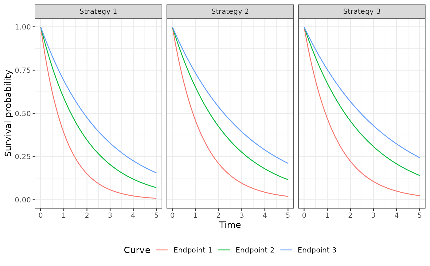
psm$sim_survival(t = seq(0, 5, 1/12))
autoplot(psm$survival_, labels = labs, ci = FALSE, ci_style = "ribbon")
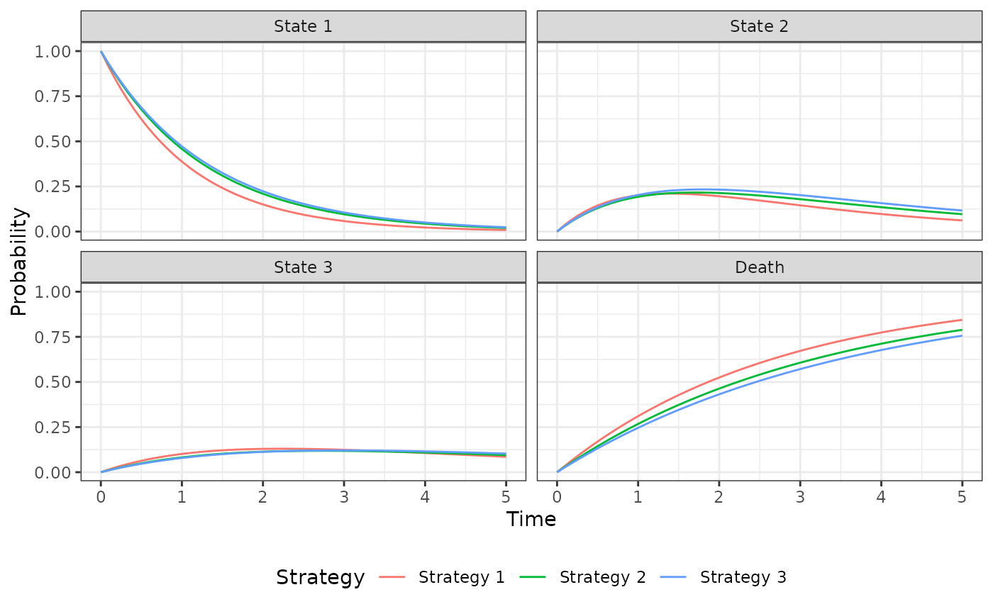
 psm$sim_stateprobs()
autoplot(psm$stateprobs_, labels = labs)
psm$sim_stateprobs()
autoplot(psm$stateprobs_, labels = labs)
 psm$sim_costs(dr = .03)
head(psm$costs_)
#> sample strategy_id patient_id grp_id state_id dr category costs
#> <num> <int> <int> <int> <int> <num> <char> <num>
#> 1: 1 1 1 1 1 0.03 medical 29233.48
#> 2: 1 1 1 1 2 0.03 medical 18094.74
#> 3: 1 1 1 1 3 0.03 medical 18303.92
#> 4: 1 1 2 1 1 0.03 medical 29233.48
#> 5: 1 1 2 1 2 0.03 medical 18094.74
#> 6: 1 1 2 1 3 0.03 medical 18303.92
head(psm$sim_qalys(dr = .03)$qalys_)
#> sample strategy_id patient_id grp_id state_id dr qalys lys
#> <num> <int> <int> <int> <int> <num> <num> <num>
#> 1: 1 1 1 1 1 0.03 0.8195100 1.0057465
#> 2: 1 1 1 1 2 0.03 0.4613371 0.6510768
#> 3: 1 1 1 1 3 0.03 0.3417771 0.5088290
#> 4: 1 1 2 1 1 0.03 0.8195100 1.0057465
#> 5: 1 1 2 1 2 0.03 0.4613371 0.6510768
#> 6: 1 1 2 1 3 0.03 0.3417771 0.5088290
psm$sim_costs(dr = .03)
head(psm$costs_)
#> sample strategy_id patient_id grp_id state_id dr category costs
#> <num> <int> <int> <int> <int> <num> <char> <num>
#> 1: 1 1 1 1 1 0.03 medical 29233.48
#> 2: 1 1 1 1 2 0.03 medical 18094.74
#> 3: 1 1 1 1 3 0.03 medical 18303.92
#> 4: 1 1 2 1 1 0.03 medical 29233.48
#> 5: 1 1 2 1 2 0.03 medical 18094.74
#> 6: 1 1 2 1 3 0.03 medical 18303.92
head(psm$sim_qalys(dr = .03)$qalys_)
#> sample strategy_id patient_id grp_id state_id dr qalys lys
#> <num> <int> <int> <int> <int> <num> <num> <num>
#> 1: 1 1 1 1 1 0.03 0.8195100 1.0057465
#> 2: 1 1 1 1 2 0.03 0.4613371 0.6510768
#> 3: 1 1 1 1 3 0.03 0.3417771 0.5088290
#> 4: 1 1 2 1 1 0.03 0.8195100 1.0057465
#> 5: 1 1 2 1 2 0.03 0.4613371 0.6510768
#> 6: 1 1 2 1 3 0.03 0.3417771 0.5088290